Contents
2. Project Background
  2.1) Introduction to traffic modelling
    Microscopic approaches
    Macroscopic approaches
  2.2) Introduction to traffic Simulation
    Examples of existing systems
  2.3) ITS (Intelligent Transport Systems)
  2.4) Introduction to straight-line geometry algorithms
  2.5) Traffic light calculations
  2.6) Animation considerations

Project Background

Simulation is used to answer "what if?" questions about things that are too complex or expensive to test for-real. Traffic systems have always come under intensive investigation using modelling and simulation. Simulation can be defined as "a dynamic representation of some part of the real world achieved by building a computer model and moving it through time" [15]. The model describes a particular abstraction of the proposed or real-world system and is built in the initial effort of comprehending the system. There are 4 components that, when brought together by a model, result in a visual simulation:

Model: This is a merger of physical laws of the objects involved in traffic systems, theory of traffic systems and the layout of the traffic network. Data: The statistics and information that will be applied to the model. Simulation: The simulation system calculates vehicle movements of cars (or whatever else e.g. trams, bicycles, pedestrians) with their specific acceleration and deceleration behaviour. Animation: The animation represents simulation results as movements of vehicles at the computer screen. Thus, simulated traffic is easy to observe and to evaluate. Validation: Validation is necessary to fit the model and data to real traffic situations (to make the simulation realistic).

Examples of uses of traffic simulation and modelling:

• To help make planning decisions by assessing risks, costs and benefits of a new traffic proposal.
• The analysis and study of different variations within traffic planning projects.
• To uncover "black spots" (Dangerous or particularly congested areas) and propose solutions.
• Optimisation of local and co-ordinated traffic light control systems.
• Detection of bottlenecks.
• The analysis of interactions of different kinds of traffic.
• To provide traffic predictions.
• Pre-emption projects for public transport.

2.1. Introduction to traffic modelling

Traffic models fall into two categories: Microscopic approaches and Aggregated macroscopic approaches.

Microscopic approaches

• To obtain a better understanding of the driver-vehicle system behaviour which can lead to the development of new safety devices.
• To provide the basic component of microscopic simulation models which test or improve new traffic control strategies.

The general form of car-following models can be represented by the stimulus-response reaction at time t:

• T is the reaction time of the driver-vehicle system.
• Response is usually de-acceleration.
• Stimulus is the difference in velocity between the lead car and the follower.

I.e. The response of successive drivers in the traffic stream is to accelerate or decelerate in proportion to the magnitude of the stimulus at time t after a time lag T.

Basic Driver Perception-action Process [18]

Car-following models applied to a number of successive vehicles are capable of describing the movement of a long string of vehicles. To simulate a multi-lane road additional modules describing lane changing or overtaking can be added to the microscopic model. Example pseudo-code:

function vehicle_updating (vehicle v) {
	if (vehicle v is at a junction) {
		apply junction-movement model;
	} else {
		if (vehicle v has to change lane) {
			apply lane-changing model;
		} else if (vehicle v has not changed lane) {
			apply car-following model;
		}
	}
	update statistics;
}

At junctions a vehicle can consult a gap-acceptance model to calculate whether or not it is safe to pull-out into the junction and continue its journey. As a model incorporates more and more real-life behaviour, the simulation that will use the model becomes capable of more and more realism.

Aggregated macroscopic approaches

• Flow (or volume) refers to the distribution of the vehicles in time. (vehicles per hour)
• Concentration (or density) refers to the distribution of vehicles in space. (vehicles per kilo-meter)
• Occupancy refers to the proportion of time a vehicle is in a particular place. It is usually measured by an induction loop buried under the surface of the road that can detect when a vehicle is above it.
• Time-mean-speed refers to arithmetic mean of the instantaneous speeds of the vehicles passing a given point during a given time period.
• Space-mean-speed refers to the arithmetic mean of the instantaneous speeds of the vehicles on a given length of road at a given instant.

Traffic density is related to traffic volume by a relationship known as the "fundamental diagram" (under homogeneous traffic conditions in space and time). The fundamental diagram provides maximum flow at a critical density value. If density is further increased (e.g. due to entering traffic), traffic volume decreases and a more or less severe congestion results.

Early theoretical road traffic studies tried to establish analogies with physical laws of incompressible fluids. The analogy only worked for high concentrations of traffic but the "kinematic wave theory" helped to model some traffic phenomena such as bottlenecks and "shock waves".

Kinematic waves are pressure waves in fluids. The consideration of a hydrodynamic theory of traffic, suggested by fluid flow analogies, has proved significant and has enabled several traffic control practices to be improved [1]. Hydrodynamic theory is based on three fundamental principles:

1. The continuous representation of variables (flow variables).
2. The law of conservation of mass (the same number of cars enter a road section as leave it).
3. The statement of fundamental design (traffic speed is a function of traffic concentration).

Shock waves can be explained by kinematic wave theory. They form in heavy traffic when drivers tend to drive too close to the vehicle in front, so there isn't enough time to react smoothly when confronted with heavy braking. In this case, if one following vehicle slows down slightly, the next has to brake harder, the next harder still, and so on. This is a case of oscillation with positive feedback. With any luck, the cycle is broken if one driver has had the sense to leave a bigger gap. In the worst circumstances the cycle is broken by a crash. [9]

Macroscopic models are capable of describing the dynamic evolution of traffic flow on long roads and traffic networks, they are used for purposes of prediction and also for models of fuel consumption.

2.2. Introduction to traffic simulation

An example of the latest animation quality on WATSIM by KLM Associates [5]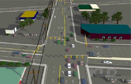

Examples of Commercial Traffic modelling and simulation tools. [4,5]

Motorway (Freeway, Corridor) Traffic Modelling
Motorway simulations have been popular due to the high traffic densities and problems of congestion making them the most cost-effective type of traffic-simulation. SCOT (Simulation of COrridor Traffic) evaluates control policies along urban freeway corridors. MicroSIM micro-simulator simulates the German freeway-network at least in realtime using parallel computation techniques. SIMAUT simulates freeways and on and off ramps based on the hydrodynamic theory of traffic flow (Macroscopic simulator). CORFLO (CORridor FLOw) was designed to simulate traffic on various types of roadways (urban streets, arterials and freeways) at a macroscopic level of detail.

Urban Traffic Modelling
Urban traffic simulators have been used to model urban congestion. They have to cope with large numbers of vehicles and signalled junctions.
NETSIM (Network Simulation) is used to help traffic engineers analyse potential urban traffic system designs.
SIMNET simulates the simplified movement of individual vehicles in connected street networks.

Intersection Design Simulations
The design of intersections is a complex problem that is important to get good traffic flow results.
TEXAS (Traffic Experimental and Analytical Simulation) helped with the need to redesign Texas highways and street systems due to the complexity of intersection design.
TRAFFICQ developed for the UK Department of Transport is designed to aid the evaluation of alternative traffic management plans for networks. SIGART was developed to extend knowledge of roundabouts and the development of signal-controlled roundabouts.

Rural Traffic Modelling
Rural simulators are less common because they are less cost effective than urban simulators. Rural simulators pay particular attention to models of road slopes and over-taking behaviour.
ROADSIM (Rural road Simulator) microscopically simulates the movement of vehicles along two lane two-way rural roads.

Signal-Timing and control system Simulations
Traffic signal control is a system for synchronizing the timing of any number of traffic signals in an area, with the aim of reducing stops and overall vehicle delay or maximizing throughput. Traffic signal control varies in complexity, from simple systems that use historical data to set fixed timing plans, to adaptive signal control, which optimizes timing plans for a network of signals according to traffic conditions in real-time. With the increase in population size, historical data for traffic-light timing information becomes obsolete within a year [13].
SIGOP II (SIGnal OPtimization) is a traffic signal optimisation model. It is designed to generate optimal traffic signal timing plans for arterial or grid networks.
CYRANO (CYcle-free Responsive Algorithm for Network Optimization) is a traffic signal optimisation model for real time traffic control. It generates network signal timing plans for undersaturated conditions. [6]
DYNEMO is used for the development, evaluation and optimisation of traffic-control systems for urban networks.
FLEXSYT (flexible network and traffic control simulation study tool) is a tool that uses a traffic control programming language (TRAFCOL) developed by Dutch traffic engineers in the study of traffic control programs.

Public-Transport Traffic Modelling
As a response to a government initiative for public transport, simulations have made attempts to find more efficient routes for public transport vehicles. AVM is a model developed to simulate the operation of buses equipped with automatic vehicle monitoring systems. Buses were simulated moving through a background traffic stream; stopping to discharge and pick up passengers; and responding to in-vehicle displays informing the driver of his schedule adherence.
TRAF-NETSIM was used to develop an adaptive bus priority system [7]
MISSION facilitates general traffic, bus, trams, light-railways for analyse of public transport systems and noise levels.

Traffic Congestion Simulations
Congestion is the main target of investigation by many simulations. Long queues can entrap cars that do not wish to pass through the bottleneck that generated them, compounding the problem and causing spillovers. Congestion management is aimed at queue avoidance and containment.
ACCESS (Area-wide Control of Congested System) is a computer model which implements a critical intersection control and queue management policy for saturated network condition.
INTRAS (Integrated Traffic Simulation) is used for the detection of stopped vehicles and the necessary steps required to remove the stoppage. It helped to develop freeway incident detection techniques for the Federal Highway Administration.

Evacuation Simulations
IDYNEV (Interactive DYnamic EVacuation Model) was developed for the Federal Emergency Management Agency. It is used to develop evacuation plans and to estimate evacuation times in response to natural and technological disasters.
TRAD (Traffic Routing and Distribution) is designed to route traffic from areas at risk to the periphery of an emergency planning zone so as to minimize evacuees exposure to risk.

Environmental Simulations
Governments and environmental agencies are often interested in fuel-consumption and emission rates made by traffic vehicles.
The TRansportation ANalysis SIMulation System (TRANSIMS) is a set transportation and air quality analysis and forecasting procedures developed to meet the Clean Air Act. [14]

Graphical Traffic Simulations
Many modern simulations now have a graphical front end.
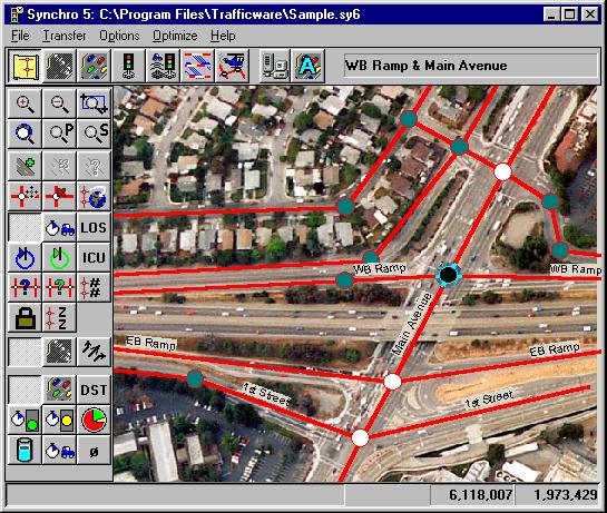
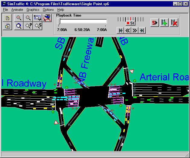
GTRAF (Graphic TRAFfic) was designed to offer the user of the NETSIM and CORFLO simulation models a graphical means of displaying results. The package include traffic animation capabilities as well as static displays, graphs, and "snapshots" of system status at user-specified times. Examples of graphical displays:

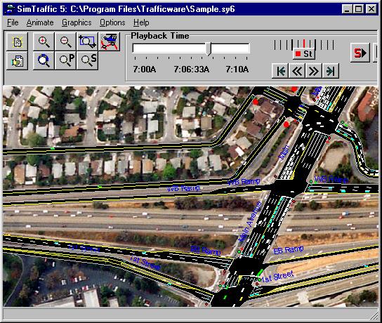SimTraffic 5.0 by TrafficWare.

SHIVA: Simulated Highways for Intelligent Vehicle Algorithms. Investigators: Rahul Sukthankar and John Hancock.

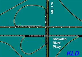WATSim simulation of proposed design for a freeway/arterial interchange in Howard County, Maryland performed by KLD Associates, Inc. LogixProTraffic Control Lab. "Utilizing TON Timers"

2.3. ITS (Intelligent Transport Systems)

Example uses of ITS:

• Traffic management tools to ensure maximum efficiency of the road network, including:
  • Monitoring current and predicting traffic conditions.
  • Co-ordinating traffic signals to minimise delays and queues.
  • Giving 'green waves' through traffic signals.
  • Improving emergency vehicle response times.
  • Detection and management of incidents on the highway network.
• Electronic payment, access control and enforcement systems, such as:
  • Automatic tolling.
  • Vehicle recognition and restriction.
  • Camera systems for traffic signal and speed enforcement.
  • Video surveillance.

The technology of the hardware and software that ITS uses can be very advanced:

• Many road-junctions today are fitted with an induction loop under the surface of the road that can detect whether a car is above it. An inductive loop is simply a coil of wire embedded in the road's surface. Inductive loops work by detecting a change of inductance caused by large steel objects positioned in the loop's magnetic field. Signal junctions of this kind are called "vehicle-actuated" because the junction knows where cars are waiting.
• Signals and pelican crossings can be synchronised by a central computer which carries out continuous calculations to determine the most efficient settings to assist traffic and pedestrian movements.
• Traffic management systems can be connected to the internet so commuters can top into real-time traffic data before they leave their driveways. [16]
• Closed Circuit Television (CCTV) images can be transferred directly to a central control room where operators are able to identify causes of congestion and intervene through control systems. Many councils currently use this system.
• A Global Positioning Satellite (GPS) bus location and priority system could enable buses fitted with on board bus units to gain priority at traffic signals. The system also could allow real-time passenger information to be displayed at bus stops to inform passengers when a bus is due.
• TV surveillance cameras for the detection and prosecution of motorists speeding or violating red lights at signals are now becoming increasingly widespread.
• Variable Message Signs (VMS) are increasingly being used to display car parking information, congestion and road weather conditions.
• Recognition software used on CCTV images could start to automate congestion corrective measures. Fixed traffic cameras have a constant background and therefore it is easier to detect moving objects for image recognition techniques.
• In the event of a system failure, the system can notify the appropriate engineers and then fall back on "baseline" information.

Many benefits are obtained from the implementation of an effective Urban Traffic Control (UTC) system, not only for traffic in the town or city involved but also for the local economy and environment [10]. These benefits are well proven and include:

• Substantial savings in journey times
• Reduction in the number of stops, leading to smoother traffic flow and reduced congestion.
• Greater fuel economy and reduced environmental pollution
• Fewer accidents due to less driver frustration
• Greater safety for pedestrians at regular crossing places
• Easier adjustment of traffic signal timings as traffic patterns change
• Improved monitoring giving instant reports of traffic signal failures
• Quicker fault detection and response
• Reduced journey times for emergency vehicles

Traffic simulations are used to develop, evaluate and optimise ITS software systems.

2.4. Introduction to simple straight-line geometry algorithms

A line joining (x1, y1) and (x2, y2) can be specified by the equation:
(y-y1)/(x-x1) = (y2-y1)/(x2-x1)

The gradient of the line is:
m = (y2-y1)/(x2-x1)

The equation can therefore be simplified to:
y-y1 = m(x-x1)

If a road is represented by the equation of a straight-line, a junction will occur when two lines intersect.

Line 1 equation: y-l1y1 = l1m(x-l1x1)
Line 2 equation: y-l2y1 = l2m(x-l2x1)

At the intersection point the two lines will have the same value of x and y. This point can be found by solving the simultaneous equations:

x = (l2m*l2x1 +l1y1 - l1m*l1x1 - l2y1)/(l2m-l1m)
y = l1m(x-l1x1) + l1y1

A car driving along a road will need to know the angle the road is at so the original image can be rotated to be orientated correctly:

In the diagram: tan(a1) = m1 and tan(a2) = m2
whilst:
Q = a1 -a2
tan(Q) = tan(a1-a2)
tan(Q) = (tan(a1) - tan(a2))/(1+tan(a1)*tan(a2))
tan(Q) = (m1-m2)/(1+m1*m2)

In particular if the lines are perpendicular, then: Q = 0.5PI and m1*m2 = -1

So to draw a car on a road of gradient m the car image must be rotated tan-1 m.

A cars new location after a moving a certain number of pixels in any direction can be calculated using the Pythagoras theorem. If Q is the angle between the x-axis and the direction of the car:

For a car to know how far away it is to another car the distance of two points needs to be calculated:
distance = sqrt(sqr(dx)+sqr(dy)) where dx = x2-x1 and dy = y2-y1.

The speed of a car can be calculated from: speed = distance/time

The acceleration of a car is its change in speed in time:
acceleration = change in velocity/time

2.5. Traffic light calculations

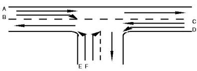Here is a T-junction with 6 routes that a vehicle can take (A-F) [11]

A set of routes is conflict-free if no pair of members of the set conflict with each other. Travel on such a set can be allowed concurrently without danger of collision.
The aim is to find maximum conflict-free sets:

Model the junction as a directed graph	List all junction routes	Conflict Diagram
	A = 1-2-3 B = 1-2-4 C = 3-2-1 D = 3-2-4 E = 4-2-1 F = 4-2-3

Conflict free sets are sets of routes not connected in the conflict diagram. Maximal conflict free sets: {A,B,E}, {A,C,D}, {A,D,E},{D,E,F}

Example solution for a signal phase: {A,C,D},{A,B,E}, { D,E,F}. This enables every route once in the cycle, with routes A,D,E (which have less conflict) getting longer phases, and with each phase representing maximal conflict-free traffic flow. Calculating optimal timing intervals for each phase depends on the traffic flow through the routes.

2.6. Animation considerations

Simulations often therefore have a "back-end" and a "front-end":

• The back-end calculates precise values for traffic vehicle locations.
• The front-end uses data from the back-end to calculate the relevant screen display.

The back-end simulation will run according to a time dimension which all members of the simulation will be synchronised to. The front-end should update the screen to show vehicle locations at a particular point in time. Animation will be caused by the front-end updating the screen as often as possible (each new time the display will be slightly different).

Double-buffering is a technique to reduce screen flicker. Using double-buffering you draw each frame of an animation off-screen, then copy the frame onto the screen all at once. The eye doesn't see any of the individual parts of the screen being drawn and so it doesn't seem to flicker.